
Software

Mastering Excel 2013's advanced formulas and functions can transform raw data into actionable insights. These seven powerhouse techniques will elevate your spreadsheet skills, automate complex tasks, and help you work like a seasoned data analyst—even if you're a beginner.
Array Formulas for Multi-Conditional Data Analysis
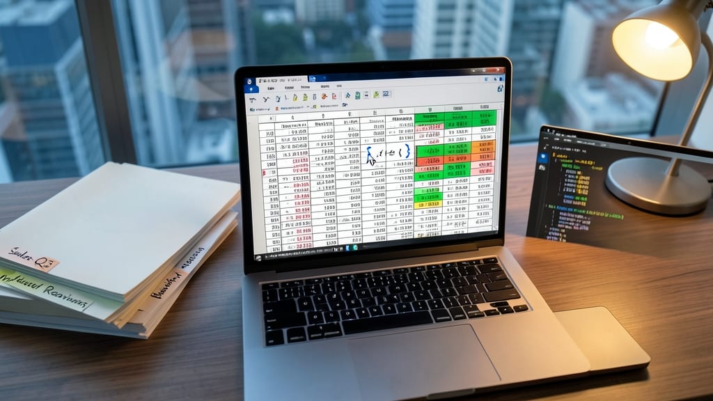
Stuck juggling multiple conditions in Excel 2013 that traditional functions like SUMIFS can’t handle? Array formulas unlock powerful calculations without requiring VBA—think of them as Excel’s built-in "supercharged logic" for complex datasets.
To use them, wrap your formula in curly braces { } (e.g., {=SUM((A2:A10>50)(B2:B10="Yes"))}) to evaluate entire ranges at once. This lets you perform multi-condition sums, averages, or counts in a single step—ideal for financial modeling where you need to filter by revenue and* region simultaneously. Unlike helper columns, array formulas recalculate automatically when data changes, making them perfect for large-scale reporting where precision matters.
Financial analysts and data teams will love this for automating complex logic—no coding required. Just remember to press Ctrl+Shift+Enter to activate the array (Excel 2013’s default behavior). ⚡
Advanced Lookup Techniques Using INDEX MATCH
Say goodbye to the frustration of VLOOKUP errors and slowdowns—INDEX MATCH is the Swiss Army knife of Excel lookups. Unlike its volatile predecessor, this combo delivers exact matches, works left-to-right or right-to-left, and handles dynamic ranges without breaking when data shifts.
Start with =INDEX(returnrange, MATCH(lookupvalue, lookup_range, 0)) for precise results. Need to search horizontally? Just flip the ranges. For bidirectional lookups, nest two INDEX MATCH formulas—perfect for cross-referencing tables where VLOOKUP fails. The real game-changer? It’s faster on large datasets and never requires column adjustments.
Data analysts, inventory managers, and anyone juggling multi-table datasets will love this for its reliability and flexibility—no more #N/A headaches or manual tweaks. ⚡
Dynamic Named Ranges for Flexible Formulas

Frustrated by formulas that break every time your dataset grows? Dynamic named ranges in Excel 2013 solve this by automatically expanding to include new data—no manual adjustments needed. Unlike static ranges, these adapt to your growing tables, making them perfect for pivot tables or complex formulas that reference entire columns.
To create one, use the Name Manager and define a range like ="SalesData"!A2:INDEX(A:A,MATCH(9.99999999999999E+307,A:A)), which captures all values until a blank cell. This works seamlessly with SUMIFS, AVERAGE, or pivot tables, ensuring your formulas stay intact even as data expands. The OFFSET function is another trick for dynamic ranges that shift with your data.
Ideal for finance teams tracking variable-length reports or project managers updating dashboards with evolving timelines—this feature cuts hours of manual updates. ⚡
Conditional Logic with IFS and Nested IF Statements

Tired of writing long, nested IF statements that look like a tangled mess? Excel 2013’s IFS function lets you evaluate multiple conditions in a single formula—no more stacking IFs like pancakes. This game-changer simplifies logic for scenarios like grading systems or inventory alerts where thresholds matter.
The IFS function checks each condition in order and returns the first true result, while nested IFs (up to 64 levels!) handle legacy compatibility. For example, =IFS(A1>90,"A",A1>80,"B",A1>70,"C") replaces =IF(A1>90,"A",IF(A1>80,"B",IF(A1>70,"C",...)))—cleaner and faster to debug. Both methods work seamlessly with other functions like SUMIFS for dynamic calculations.
Teachers, inventory managers, and project leads will love this for clear, maintainable logic. ⚡
Text Manipulation with TEXTJOIN and SUBSTITUTE
Messy text data—like survey responses or product codes—can derail even the most organized spreadsheet. The TEXTJOIN and SUBSTITUTE functions in Excel 2013 turn chaotic strings into clean, actionable information with just a few clicks.
TEXTJOIN combines text from multiple cells into one, ignoring blank cells, while SUBSTITUTE replaces specific characters or phrases—ideal for standardizing formats. For example, merge survey answers with =TEXTJOIN(", ", TRUE, A2:A10) or clean product codes with =SUBSTITUTE(B2, "-", ""). Both functions handle delimiters and wildcards, making them versatile for reports or exports.
Perfect for marketers consolidating feedback, e-commerce teams reformatting SKUs, or analysts preparing data for external stakeholders. These tools save hours of manual editing—no VBA required! ✨
Date and Time Calculations with EOMONTH and WEEKNUM
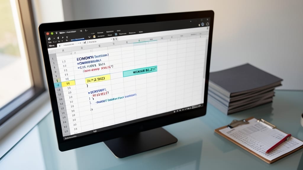
Tired of manually adjusting dates for payroll, project timelines, or inventory cycles? The EOMONTH and WEEKNUM functions in Excel 2013 automate these tasks with precision, eliminating guesswork.
EOMONTH returns the last day of a given month—perfect for calculating deadlines or end-of-month reports. For example, =EOMONTH("1/15/2023", 2) instantly gives you February 28, 2023, even if leap years complicate things. Meanwhile, WEEKNUM extracts the ISO week number from a date, ideal for scheduling or resource planning.
HR managers can auto-generate payroll cycles, project teams can align deadlines with fiscal quarters, and warehouse staff can track inventory rotations by week—all without manual date tweaking. ⚡
Error Handling with IFERROR and AGGREGATE Functions
Tired of seeing #DIV/0! or #N/A errors disrupt your spreadsheet calculations? The IFERROR function lets you replace error messages with custom text or values—like returning "N/A" instead of a broken formula.
Pair it with AGGREGATE to handle hidden rows seamlessly. AGGREGATE’s 7th function option ignores hidden cells, perfect for auditing datasets where users might filter out rows. For example, =AGGREGATE(9,6,B2:B100) skips hidden values entirely, while =IFERROR(A1/B1,"No Data") prevents division errors.
Accountants and data analysts will love this combo for clean, error-free reports—no more manual fixes or messy workarounds. ✨